Summary |
|
Automatic tracking of cells in time-lapse microscopy is required to address many biological questions. Brightfield imaging is often preferred because it limits cell-line manipulation and reduces phototoxicity during imaging. However, segmentation and tracking of cells in brightfield images is difficult, and the quality of available software is hard to assess without broadly available benchmarks and comparison methodologies. To address this gap in yeast research, we provide an annotated benchmark of yeast images covering a variety of situations, including i) single cells and small colonies, ii) colony translation and merging, and iii) large colonies with heavily clustered cells. We also provide the Evaluation Platform, a mathematically grounded tool for analysing algorithm outputs and comparing them with other available methods. We applied the platform to five software tools: Intensity Based Segmentation - Overlap Based Tracking (IBSOBT) via CellProfiler, CellTracer, CellID, Tracker, and CellSerpent. These results were later extended with the Wood2019 segmentation and tracking solution. By providing both benchmark data and a lower barrier for algorithm comparison, we enable quantitative assessment of yeast cell tracking algorithms. We encourage the community to verify these results, reuse the benchmark, and contribute additional data or algorithm outputs.
|
Introduction
Yeast is a single-celled organism that is much studied in molecular biology and genetics. As a model organism, it is used to study complex processes that occur in most eukaryotic cells by examining their counterparts in yeast. It can be grown and stored easily and its genetic material can be modified, making it an excellent experimental model.
One important application is fluorescence microscopy, where tagged proteins allow us to observe the dynamics of selected genes. These dynamics can now be studied in vivo in individual cells, unlike population-level approaches such as protein immunoblotting. To better understand biological systems, researchers often use inducible promoters triggered by osmotic shock, temperature, or chemical agents, and then observe how the system responds, for example through changes in gene expression. A related question is how these response systems are modified during inheritance.
Understanding the mechanisms that govern biological systems often requires collecting and analysing large datasets. Manual analysis is frequently infeasible, making automated computational methods necessary. The main difficulty lies in cell segmentation and tracking. Segmentation is the process of identifying individual yeast cells in images. In brightfield microscopy this is challenging because yeast cells lack strong visual hallmarks, and common microscopy artefacts such as dirt or loss of focus make the task harder. Tracking depends on segmentation, so segmentation errors propagate into tracking results. Although several software solutions have been developed for brightfield yeast analysis, their quality is difficult to assess without shared benchmarks and comparison methodologies.
In the first phase of the Yeast Image Toolkit project, we aimed to systematically compare software solutions for segmentation and tracking of yeast cells in brightfield images. To support this goal, we provide:
- an annotated benchmark of yeast images containing multiple datasets with ground truth for both segmentation and tracking
- an Evaluation Platform and methodology for quantitative assessment of segmentation and tracking algorithms
- quantitative and qualitative evaluation of five software solutions for yeast cell segmentation and tracking
Benchmark specification
We are grateful to the Grégory Batt and Pascal Hersen labs for providing the images used to construct datasets 1-7. Most images were acquired by Jannis Uhlendorf for the gene expression control project (Uhlendorf2012); some were acquired by Artémis Llamosi, who extended Jannis Uhlendorf's work.
We also thank N. Ezgi Wood, Orlando Argüello-Miranda, Andreas Doncic, and the Doncic Lab for providing both data and ground truth for datasets 8-10.
Datasets 1-5:
All datasets were recorded using a pSTL1::yECitrine-HIS5, Hog1::mCherry-hph budding yeast (Saccharomyces cerevisiae) strain derived from the S288C background. During the experiment, doubling time varied between 100 and 250 minutes.
Specification of acquisition:
- Optics: 100× objective (PlanApo 1.4 NA; Olympus). Oil immersion lenses. Images were taken with automated inverted microscope (IX81; Olympus) equipped with an X-Cite 120PC fluorescent illumination system (EXFO) and a QuantEM 512 SC camera (Roper Scientific). The YFP filters used were HQ500/20× (excitation filter; Chroma), Q515LP (dichroic; Chroma), and HQ535/30M (emission; Chroma).
- Channels:
- Channel 00: Brightfield images (50ms exposure).
- Channel 01: The fluorescence exposure time was 200 ms, with fluorescence intensity set to 50% of maximal power. Importantly, illumination, exposure time, and camera gain were not changed between experiments, and no data renormalization was done.
- Time lapse acquisition: Images in channel 00 were taken every 3 minutes, images in channel 01 every 6 minutes. Autofocus was used to find cells in channel 00 and the same Z settings were reused for channel 01.
- Benchmark construction: Five test sets (TS) were extracted from the original data.
Datasets 6-7
The yeast strain and optics were the same as in datasets 1-5.
Specification of acquisition:
- Channels:
- Channel 00: Brightfield images (50ms exposure)
- Channel 01: The fluorescence exposure time was 200 ms, with fluorescence intensity set to 12,5% of maximal power. Importantly, illumination, exposure time, and camera gain were not changed between experiments, and no data renormalization was done.
- Time lapse acquisition: Images in channel 00 were taken every 2 minutes, images in channel 01 every 2 minutes. Autofocus was used to find cells in channel 00 and the same Z settings were reused for channel 01.
- Benchmark construction: To increase variety, only every other image in the series was considered. Two test sets (TS) were extracted from the original data.
Datasets 8
Yeast cells recorded in the Doncic Lab by N. Ezgi Wood and Orlando Argüello-Miranda [1].
Specification of acquisition:
- Transmission light images, frames registered every 3 min.
Datasets 9
Yeast cells recorded in the Doncic Lab by N. Ezgi Wood and Orlando Argüello-Miranda [1].
Specification of acquisition:
- Phase contrast images, frames registered every 3 min.
Datasets 10
Yeast cells recorded in the Doncic Lab by Andreas Doncic [1]. The movie shows pheromone-treated cells with irregular morphology.
Specification of acquisition:
- Phase contrast images, frames registered every 1.5 min.
Benchmark description
Ten test sets (TS) are currently included, covering the following basic situations:
- single cells and small colonies (TS1, TS2, TS6, TS9 and TS10)
- colony translations and merging (TS3)
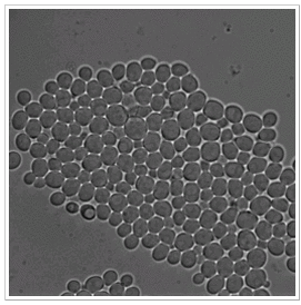
- large colonies with heavily clustered cells (TS4, TS5, TS7, TS8)
Ground truth
Automatic algorithm evaluation requires ground truth. For each test set, ground truth was prepared manually by one of the authors and then verified and corrected by the rest of the team. The resulting annotations include cell-centre locations, a unique cell identifier throughout the test set, and a "facultative" tag. The facultative tag marks cells at image boundaries, which some algorithms discard by design, as well as objects considered ambiguous. Algorithms are neither penalized nor rewarded for detecting or omitting cells marked as facultative.
Overview
The following table summarizes the test sets:
| Test set | Start time | Frame count | Cell number span | Animation |
|---|---|---|---|---|
| TS1 | 1 | 60 | 14 - 26 |  |
| TS2 | 1 | 30 | 4 - 6 |  |
| TS3 | 191 | 20 | 101 - 128 |  |
| TS4 | 225 | 20 | 171 - 237 |  |
| TS5 | 180 | 20 | 140 - 173 |  |
| TS6 | 65 | 10 | 36 - 49 |  |
| TS7 | 150 | 10 | 129 - 184 |  |
| TS8 | 1 | 30 | 60 - 88 |  |
| TS9 | 1 | 30 | 41 - 68 |  |
| TS10 | 1 | 30 | 16 - 16 |  |
Principles of the state of the art algorithms
Cell segmentation and tracking are widely studied problems that have been approached in many ways. Shen et al. (2006) presented an active-contour segmentation approach for fluorescence images combined with particle-filter tracking (Shen2006). Kvarnström et al. (2008) addressed yeast cell segmentation in brightfield images using a combination of circular Hough transform and dynamic programming on polar plots (Kvarnstroem2008). Zhou et al. (2009) proposed Markov models for segmentation and cell-phase identification in fluorescence microscopy (Zhou2009). Delgado-Gonzalo et al. (2010) introduced a probabilistic formulation of tracking on bipartite graphs and a cell-motion model dependent on neighbouring cell movements (Delgado2010). Sansone et al. (2012) combined circular Hough transform with machine-learning-based false-positive detection for phase-contrast microscopy segmentation and evaluated the algorithm using precision and recall (Sansone2012).
In 2019, we added the algorithm by Wood et al. (Wood2019). We thank the authors for providing both the description and partial results. The algorithm jointly segments and tracks each individual cell from the last frame to the first using multiple watershed thresholds.
Here we describe seven algorithms selected as best fitting our needs for segmentation and tracking of yeast cells in brightfield microscopy: CellID (Gordon2007), Intensity Based Segmentation - Overlap Based Tracking via CellProfiler (IBSOBT) (Carpenter2006), CellTracer (Wang2009), Tracker (Uhlendorf2012), CellSerpent (Bredies2011), Wood (Wood2019).
| Program | Webpage | Publication |
|---|---|---|
| Cell Tracer | http://www.stat.duke.edu/research/software/west/celltracer/ | (Wang2009) |
| CellID | http://lbms.df.uba.ar/ | (Gordon2007) |
| CellProfiler | http://cellprofiler.org/ | (Carpenter2006) |
| Tracker | upon req. | (Uhlendorf2012) |
| Cell Serpent | http://microscopy.uni-graz.at/index.php?item=new2 | (Bredies2011) |
| Cell Star | http://cellstar-algorithm.org/ | (Versari2017) |
| Wood | https://journals.plos.org/plosone/article?id=10.1371/journal.pone.0206395 | (Wood2019), (Doncic2013) |
Cell Tracer
CellTracer uses an iterative combination of morphological operations to segment brightfield and fluorescent images. The segmentation process consists of two main steps: preprocessing and cell identification. The approach introduces black-white/grayscale hybrid images, reserving the extreme values 0 and 255 for special purposes such as marking background or borders.
Preprocessing
Preprocessing partitions images into three classes: background regions, border regions, and regions still to be decided.
Background identification
Background identification uses a modified non-linear range filter with a disk-shaped structuring element. Assuming that cells are relatively smooth, the element radius is chosen between r and 2r, where r is estimated as the maximum cell half-width across processed images. After filtering, the image is thresholded with a fixed user-provided value, so pixels below the threshold are marked as background. The filter is followed by morphological dilation.
Border identification
Borders are identified using high-pass range filter. It also has disk-shaped structure element. The second significant change to default filter is that background pixels from previous step are not considered as minimum values within the neighborhood of processing pixel. For this step there is also a threshold value assuring that only obvious borders are marked - as maximum values (255) - on the hybrid image.
Cell identification
The second and main step is identification of cells in preprocessed hybrid image. It is achieved in following steps:
- Labelling disconnected blobs (disconnected segmented regions)
- Filtering each labelled blob using hybrid filters or a combination of filters, to erode the undecided regions, followed by hybrid dilation and smoothing to restore most of the pixel values changed by the filter- it leads usually to breaking down blobs into smaller ones.
- Scoring blobs based on cell model assumptions - score in two criterions:
- Cell shape - cell shapes are assumed to be convex or almost convex. Score is computed as difference between blob area and blob convex area divided by blob perimeter
- Cell intensity value distribution - interior cell regions are assumed to be relatively darker than border regions.
- Dividing blobs into two subsets - these with higher score and these with lower score
- Repeating steps 1-4 for cells with higher scores
CellID
This program was developed around the observation that images of yeast cells that are taken slightly out of focus have a very distictive dark rim around them. It makes it fairly simple to find these edges using adaptive thresholding. However in this work that specific type of imagery is not available but we will try to compensate for it with the proper preprocessing.
Cell segmentation:
Dark boundary pixels are found using a threshold with a cutoff calculated as the distribution mean minus a chosen number of standard deviations. Then cells are defined as the contiguous regions separated by these boundary pixels. The next step is filtering out the regions which sizes are outside a specified range. These preliminary results of the segmentation are then processed using simple heuristics that can split up two joined cells.
Tracking:
The newly found cells are compared with cells from previous frame based on their geometrical overlap defined as intersection over union of the cells regions. The new cell is matched with the one with the highest value only if it is above the user-defined cut off.
Intensity Based Segmentation Overlap Based Tracking (IBSOBT) via CellProfiler
Processing image sequence in CellProfiler proceeds as follows:
Pre-processing:
The first step is preprocessing image. It uses three types of images: smoothed input image, thresholded and smoothed edges image, and image with convex hull-smoothed illumination correction. Cell interiors intensities are increased by combining illumination correction image with original image, then border intensities are decreased by subtracting smoothed and thresholded edges.
Cell segmentation:
CellProfiler contains a modular three-step strategy to identify objects even if they touch each other.
- CellProfiler determines whether an object is an individual nucleus or two or more clumped nuclei.
- The edges of nuclei are identified, using thresholding if the object is a single, isolated nucleus, and using more advanced options if the object is actually two or more nuclei that touch each other (Wahlby, 2004).
- Some identified objects are discarded or merged together if they fail to meet certain your specified criteria. For example, partial objects at the border of the image can be discarded, and small objects can be discarded or merged with nearby larger ones.
Tracking:
When trying to track an object in an image, CellProfiler will search within a maximum specified distance of the object's location in the previous image, looking for a "match". Objects that match are assigned the same number, or label, throughout the entire image sequence. Here we use overlap approach that compares the amount of spatial overlap between identified objects in the previous frame with those in the current frame. The object with the greatest amount of spatial overlap will be assigned the same number (label).
'Tracker'
This algorithm, used by Uhlendorf et al. (2012), represents a model-based approach. It assumes that yeast cells are circular and therefore searches for potential circles in the image.
Preprocesing:
First the gradient field of the input image is calculated which is then thresholded to leave only pixels that are supposed to belong to the borders of the cells.
Cell segmentation:
The circular Hough Transform is used to determine the positions and radiuses of the circles representing cells. Every pixel 'votes' for all the circles it can belong to and after accumulation of all the votes the circles with locally highest vote count are chosen.
Tracking:
The cells recognized in the current image are compared with the ones from the last (or last but one if the gap is detected) image. Linear optimization is used to match the cells using a defined cell-to-cell distance matrix.
CellSerpent
Implementation of an algorithm described by K. Bredies and H. Wolinski in (Bredies2011). The main idea behind this approach is to adapt Active Contours algorithm for cell segmentation purpose.
Preprocessing
Preprocessing contains three steps:
- Background normalization
- Background detection
- Computing non-linear elliptic degenerate denoising
Segmentation
Seeding
This part of algorithm finds start points for Active Contours algorithm - "seeds" from which cells are grown up. This is done by finding the local maxima for a smoothed edge-penalization image. Local maximum usually corresponds to point in the center of a cell. Points obtained by this procedure are clustered to ensure that a minimum distance is preserved and returned after checking that none of the points lies in the previously determined cell-free-region mask.
Cell detection
This step requires its own computation of edge-penalization images for both original image and smoothed image. Additional penalization is added for the cell-free regions in order to avoid the active contour entering there. For each seed from previous step an active contour is initiated around it and evolved according to the optimization problem with edge-penalization image obtained from smoothed image. After meeting the stopping criterion, the procedure is repeated with the edge-penalization image obtained from original image and returns the contour of the cell.
Postprocessing
After the contour tracing is finished, the method creates a label image which assigns each pixel a positive natural number unique to each cell and 0 to the background. Starting with the contour associated with the lowest functional value for optimization problem, the region occupied by the contour is determined and checked against the label image for intersection. If the area of intersection is too large, the current region is rejected, otherwise, it is incorporated into the label image with a new number. In the resulting label image, each cell can be identified through the corresponding pixels.
CellSerpent*
We use this designation for our modification of CellSerpent algorithm. This designation refers to our modified version of the CellSerpent algorithm. The changes slightly improved the results compared with the original version and include:
- Enhanced background detection
- Enhanced edge continuity to prevent seeds from falling directly between two cells
CellStar
Preprocessing
In this step a background image is prepared - either predefined or manually chosen and adjusted to remove areas occupied by cells. Processed image is divided according to background image into two parts:
- pixels darker than background and its median filtered version
- pixels brighter than background and its median filtered version
Foreground content-border segmentation
Foreground regions are determined for processing image as areas where difference of values between image and background is relatively big. Then foreground is enchanced with two-step hole filling and split into two parts: content and border
- darker part is cell content
- brighter part is cell border
Seed and grow snakes
In few steps - first find big cells then try to find smaller.
Find new seeds (depends on parameters)
Based on cell content or border pixels (potentially excluding already segmented regions) and previous computations
- find local minima
- cluster minima (from CellSerpent?)
- centroids of previous snakes
Grow new seeds into snakes
Prepare uniformly distributed rays from seed position
- for different length of rays calculate its properties
- choose best length for every arc
- starting from the best arc drop the consecutive ones if the distance too big
- unstick edge points?
- an additional smoothing?
- calculate best snake properties
Filter snakes list
- sort snakes by rank
- remove snakes with too high rank
- trim snake to regions free from better snakes
- recalculate properties and remove snake if not good enough
Tracking
Find cell detection data
Collect all the centroid and size data from segmentation
Find initial cell tracks
Uses min-cost assignment (Hungarian) based on distance and size
Improve results through a few iterations
- ComputeDetailedMotion
- ComputeMotionByFrames
- GetLocalizedPrimitiveTracks
Wood
Ezgi Wood provided us with the description of the solution. The algorithm’s implementation in MATLAB is available as a supplementary material at the journal website.
The algorithm starts with segmenting the last image of a time series and segments images backwards in time by using the segmentation of the previous time point as a seed for segmenting the next time point.
Seeding last time point
The image of the last time point is automatically segmented by a two-step automated seeding algorithm: First, the image is pre-processed and watershed algorithm is applied to the processed image to generate coarse seeds. Next, the algorithm automatically fine-tunes these coarse seeds and automatically detects and corrects segmentation mistakes (Wood2019).
Stable cell contour
Next, given a seed for the cell, the algorithm focuses on a subimage containing the seed. First, the algorithm creates a series of binary images by applying every possible threshold for an 8-bit image. The watershed algorithm is applied to all these binary images and regions that significantly overlap with the seed are combined in a composite image that allows for more accurate segmentation than one optimized threshold (Doncic2013).
Tracking
The cells are tracked based on their overlap with their seed.
Input data assumptions
Every algorithm has to make some assumptions about the input data and what cells generally look like so it can utilize this in cell segmentation. We sum up these basic assumptions in the following table:
| IBSOBT via CellProfiler | CellTracer | CellID | Tracker | CellSerpent | CellStar | ! Wood |
|---|---|---|---|---|---|---|
| Bright and thick borders | Brighter borders, darker content / background * | Dark borders | High gradient borders | High gradient borders | Brighter borders, darker content compared to background | Brighter borders, darker content ** / background |
*There is a possibility to invert input values in CellTracer's GUI. **If the content is not dark, a composite image of phase and fluorescent image can be used for segmentation.
Specification of dataset adjustments and tool configurations
Comparing existing tools poses several challenges. In image processing, algorithm performance strongly depends on the data used. A simpler and theoretically weaker method can outperform more complex methods on very noisy input images.
Another challenge is that the compared tools are configurable, so the chosen configuration may not be optimal. Algorithms may also require suitable preprocessing to enhance the image features they rely on. A fair comparison therefore requires testing both configurations and preprocessing choices.
Our solution is to start the search for the best preprocessing-configuration pair using the remarks in the corresponding papers. Then for every test set we try to adjust the parameters to produce better results.
The following sections describe both the preprocessing used and how the 'optimal' configurations were determined.
Cell Tracer
Image preprocessing:
Contrast enhancement.
Configuration determination:
The optimal configuration was obtained by choosing the right combination from a small predefined set of methods grouped by purpose: background detection, border detection, cell identification, and tracking. The configuration combined methods in this order. For each method, specific parameters were adjusted until the output was satisfactory. Methods within each group were tested in different orders to find the best solution. Tests were performed on 2-3 images per dataset and the results were visually checked against the requirements. We used saved snapshots after obtaining good results for one method, avoiding repetition of the whole previously adjusted sequence before each parameter change in the currently tested method.
CellID
Image preprocessing:
Smoothing, inversion, contrast enhancement, unsharp filtering, and optional minimum morphology.
Configuration determination:
This tool is designed for out-of-focus images, which is not the case here, so we mimic the relevant characteristics through preprocessing. To create dark rims, we invert the image and use a combination of contrast enhancement and an unsharp filter to enlarge them. For test sets with highly clustered cells, we additionally apply minimum morphology for better separation.
The optimal parameters were chosen per data set using one of its images. First the acceptable cell size was selected so that every possible cell is valid and the small incorrect ones are filtered out. Then the background reject factor and the rest of the parameters were trimmed to find the balance between separation of clustered cells and oversegmentation of the existing ones.
IBSOBT via CellProfiler
Image preprocessing:
Smoothing, contrast enhancement, and edge enhancement.
Configuration determination:
Optimal configuration was obtained during two stages - local and global. Both stages were performed on 2-3 images. In the first stage, the output of each pipeline module was visually compared with the expected output, and parameters were corrected until a satisfactory result was obtained. In the second stage, parameters were adjusted to improve later modules, especially the final segmentation and tracking steps.
'Tracker'
Image preprocessing:
Contrast stretch
Configuration determination:
The optimal configuration was obtained by choosing the right parameter-preprocessing combination. The test image was preprocessed in several ways, including median filtering, contrast stretching, and equalization. For every dataset, the image most challenging for the default parameters was used for parameter tuning. First, a sensible cell-size range was set. Then the threshold and filter-radius parameters were adjusted until the best results were obtained.
CellSerpent
Image preprocessing:
Edge enhancement
Configuration determination:
Optimal parameters were determined for each stage separately and then confirmed to work well in combination. This was done by visually rating the results of image smoothing, background determination, and seeding, followed by both visual and automatic evaluation of the active-contour algorithm.
CellStar
Image preprocessing:
None (for our test sets).
Configuration determination:
Default configuration
Wood
Algorithm was applied to test sets TS1-2, TS6, TS8-10.
Image preprocessing:
Brightfield images were first corrected for uneven background by subtracting a Gaussian-filtered image. Next, a top-hat transformation was applied. For TS8, complements of the brightfield images were used. Phase images were not processed.
Configuration determination:
The optimal configuration was obtained by choosing the right processing for brightfield images and optimizing parameters for the objective magnification and imaging conditions. Brightfield images were processed to make borders brighter than cell centres and background. To optimize parameters, the last image of the time series was used: it was first segmented with default parameters and then adjusted until a satisfactory output was obtained. For implementation details and parameter values, see (Wood2019).
Result of the comparison
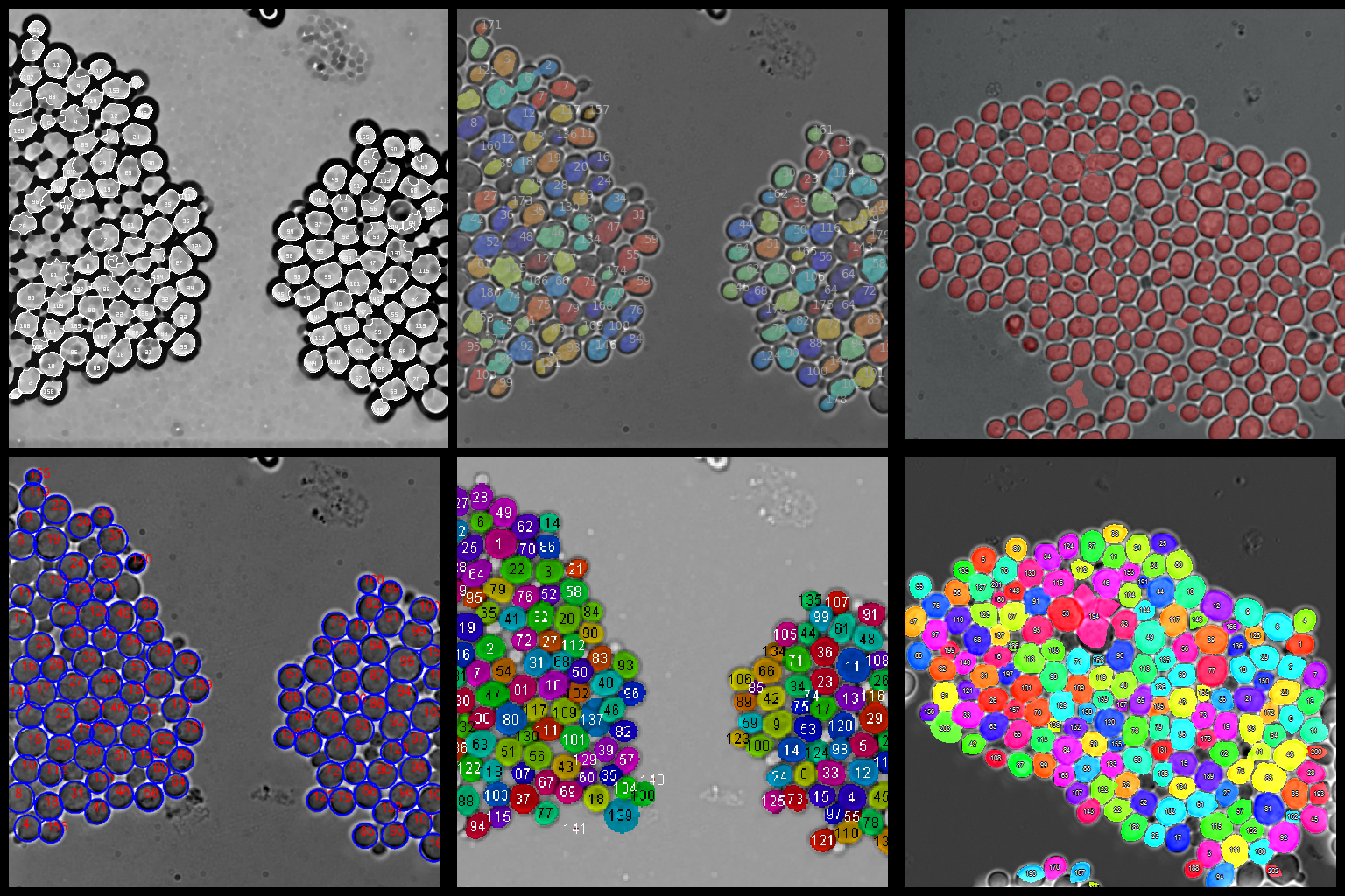
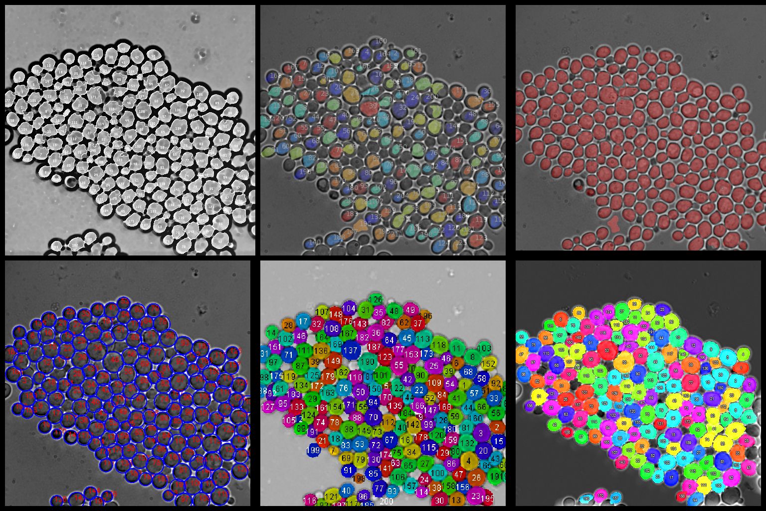
Visual inspection:
The first comparison method is visual inspection. To make inspection more accurate and convenient, we arranged the results in a 3 by 2 grid.
Undersegmentation
Undersegmentation appears in almost every tested program, with 'Tracker' as the only exception. It occurs when a region detected as one cell contains areas belonging to several cells. In the programs where it appears, it is very rare.
Examples of undersegmentation
Oversegmentation
Oversegmentation similarly appears in every program except 'Tracker'. In contrast to undersegmentation, it occurs when one cell is detected as several cells. It is rare for CellStar and CellSerpent, appears more often in IBSOBT than in CellTracer, and is most frequent in CellID.
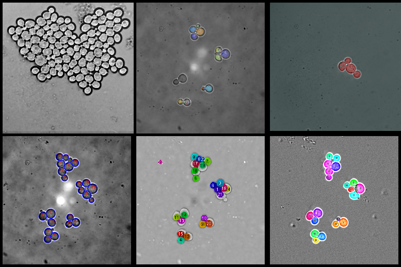
Examples of oversegmentation
False positives
No tested program is free of false positives. However, 'Tracker' and CellStar produce very few false positives, mostly in noisy background regions. CellTracer and IBSOBT detect false positives in areas between groups of cells; CellID finds many cells in noisy background; and CellSerpent suffers from imprecise background detection, causing seeds to fall outside areas covered by cells.
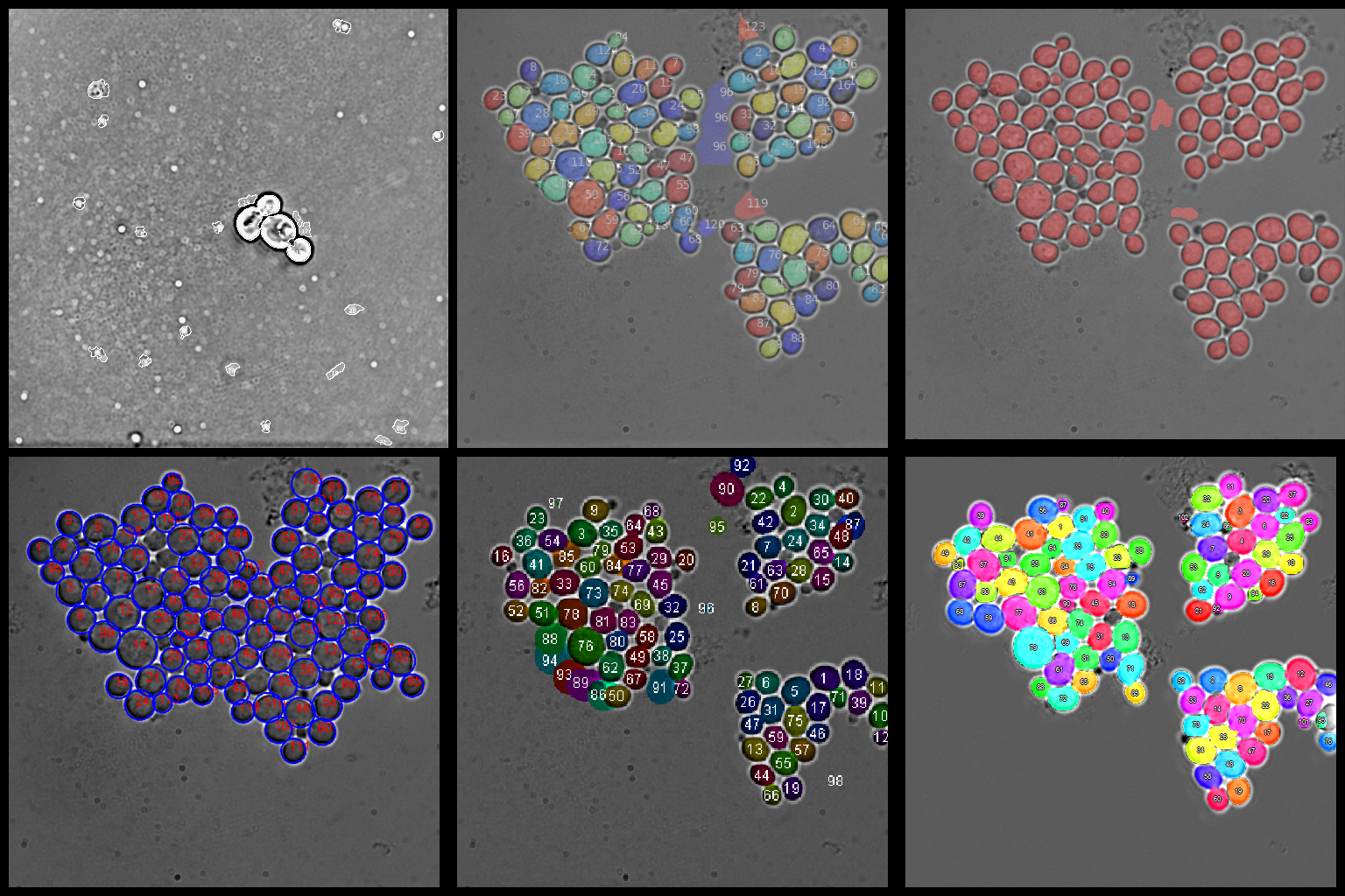
Examples of false positives
False negatives
False negatives are among the most important obstacles in downstream cell processing. CellStar is the clear leader, omitting cells least often, while CellTracer also performs well. Other programs produce more false negatives, especially IBSOBT, most likely because of inconsistent cell interiors.
Examples of false negatives
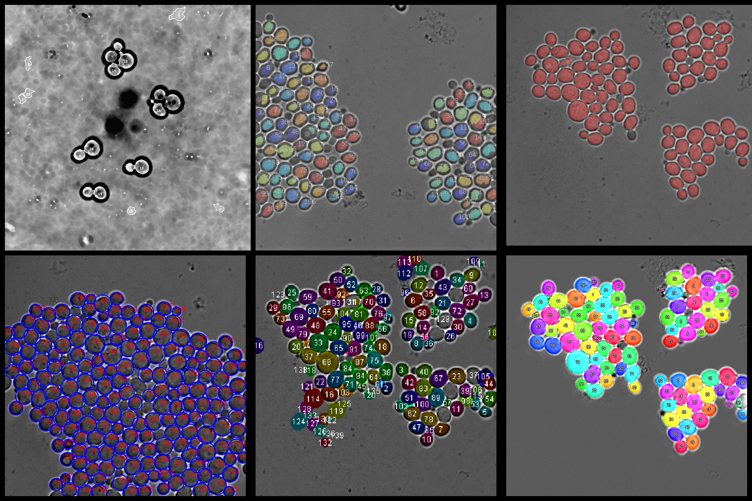
Cell contour extraction accuracy
The tested programs use different cell-contour extraction techniques, but in most cases the contours are extracted quite accurately. The exception is Tracker, which uses circular Hough transform and therefore extracts cell contours as circles.
Examples of cell contours extraction
Detection of cells near image boundaries
Because of their specific image-processing techniques, some programs miss cells near image boundaries. CellTracer has the fewest problems with this issue, while Tracker and CellSerpent also cope with it relatively well.
Detection of cells near image boundaries
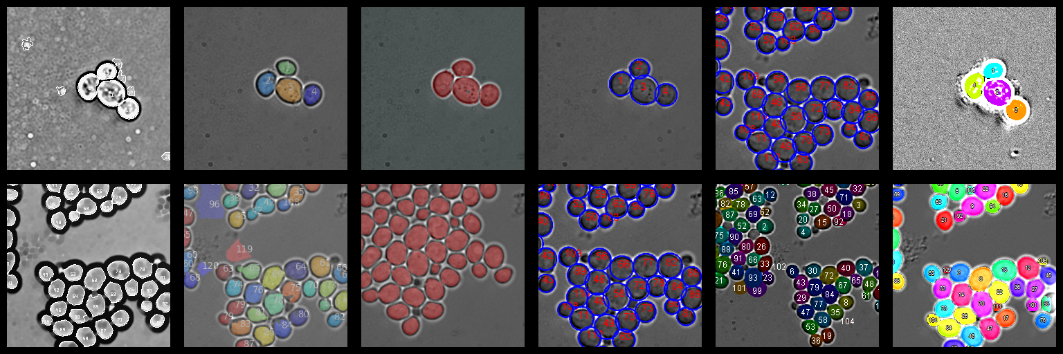
Detection rate for new cells
From the perspective of lineage analysis, detecting new cells is probably the most important issue. CellStar performs best among the tested programs. One drawback is that the technique enabling early detection of new cells may cause oversegmentation in some cases. CellTracer performs almost as well, although its side effect is false-positive detection. CellID and CellSerpent detect new cells within a reasonable time, but not as quickly as CellStar or CellTracer. Tracker and IBSOBT perform poorly: Tracker has a five-frame latency compared with CellStar, while IBSOBT has an even longer delay, as shown below.
Detection of new cells
Tracking errors
No program tracks cells perfectly. The example below shows a very challenging situation in which none of the tested programs tracks cells without errors. CellSerpent does not provide cell tracking, so no visual result is shown for it.
A problematic situation for tracking
Summary
It is apparent that none of the algorithms is perfect: all of them miss some cell regions. CellStar is the most successful because it marks almost every cell and almost never detects a cell where none exists, whereas the other methods struggle with clustered cells and spaces between cell groups. Together with CellTracer, it also has the best budding-cell detection rate. On the other hand, CellTracer is the only algorithm with no visible problems detecting cells near image boundaries.
Automatic evaluation:
Manual evaluation should be supplemented by automatic evaluation. Here, both segmentation and tracking results can be tested against manually created ground truth. The first step is to find correspondences between ground-truth cells and cells in the algorithm output. This can be achieved using a simple nearest-neighbour method or a more sophisticated linear-programming approach (Sansone, 2011).
Quality measures:
Several conceptually similar segmentation quality measures are used:
- False positive/negative (Bao, 2007)
- Oversegmentation/undersegmentation (Wählby, 2004 and Zhou, 2006/2009)
- Precision/recall (Sansone, 2011)
A false-positive is a cell that is recognized by the algorithm but does not exist in the ground truth. A false-negative is a cell that the algorithm missed. All the rest is simply a variation of that. Precision and recall measures are used in this work as they are normalized by the total cell number. It is important to consider both measures because an algorithm can often be tuned to increase one at the cost of the other.
Precision and recall calculation method:
Let R be the set of cells in the results, G be the set of cells in the ground truth and C be the set of correspondence pairs between R and G. Then:

F is an additional quality measure (combining precision and recall).
The above measures test only the ability of the algorithm to find the centers of cells so to evaluate the accuracy we can calculate the overlap of the corresponding contours (Sansone, 2011). However in this paper it is done by visual inspection.
Facultative ground truth:
There are some inconclusive objects in the images and the algorithms should not be penalised nor rewarded for finding them, otherwise it would clutter the results.
Let  be the set of cells in the ground truth marked as facultative.
Then:
be the set of cells in the ground truth marked as facultative.
Then:

Precision and recall can then be properly adjusted:
Tracking evaluation
Tracking performance in each image can be evaluated using similar precision and recall measures based on the number of correct links (Primet, 2011). A link consists of two consecutive points in a cell trajectory. A correct link occurs when the algorithm finds both points in the ground truth and recognizes that they belong to the same cell.
Precision, recall, and F are calculated analogously to segmentation, but with:
= the subset of C where at least one end is marked as facultative
Another measure for tracking performance is long-term tracking which evaluates the ability of the algorithm to correctly track cells throughout the whole image series. For this purpose we adapt the tracking measure defined above. It is calculated for the set of only two images (first and last).
Evaluation platform:
The previous section presented measures viable for evaluation of image segmentation and tracking. In order to apply these measures to benchmark test sets, we created the Evaluation Platform, a Python package for quantitative assessment of cell segmentation and tracking results against ground-truth annotations. The platform was developed for Yeast Image Toolkit, but the evaluation logic is not yeast-specific and can be used with other cell-tracking datasets.
The platform provides command-line tools for evaluating a single algorithm, comparing multiple algorithm outputs, and evaluating individual frame pairs for feedback-loop or parameter-search workflows. It supports center-based annotations as well as label- or mask-based segmentation results, computes segmentation, tracking, and long-term tracking scores, and can generate summary reports, CSV tables, F-score plots, and optional visual overlays marking correct detections, false positives, and false negatives on the input images. The maintained version is available at https://github.com/Fafa87/EP.
Results:
Test set 3 is very challenging for tracking because three different yeast colonies suddenly merge, so we start with this case. First, let us examine segmentation performance. All algorithms performed well, with more than 85% of cells found and precision above 90%. The best results were achieved by CellStar, with over 95% of cells detected and almost all returned cells correct.
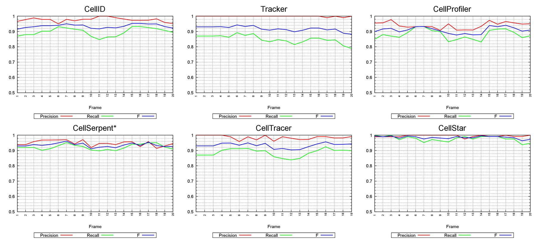
Segmentation evaluation in TestSet3.
In the case of this test set tracking evaluation is much more interesting. It is clear from the plots when movement occurs. Only CellStar is able to cope partially with this situation, because the other algorithms use overlap or distance between cells for tracking, which is not meaningful in this case. A better solution would use cell-based characteristics such as size, shape (Zhou, 2006, 2011), or even intensity histograms. Another improvement would be to account for the relative position of a cell and its neighbours, which usually does not change dramatically and is used by CellStar.
Tracking evaluation in TestSet3.
Table summarizing segmentation quality (F measure) in all TestSets (green - best; blue - second best, NE - not evaluated):
| Test set | IBSOBT | CellTracer | CellID | Tracker | CellSerpent* | CellStar | Wood |
|---|---|---|---|---|---|---|---|
| TS1 | 0.8847 | 0.9239 | 0.6302 | 0.9351 | 0.9712 | 0.9921 | 0.9894 |
| TS2 | 0.8923 | 0.9071 | 0.3073 | 0.9531 | 0.9677 | 0.9895 | 1.0000 |
| TS3 | 0.9094 | 0.9331 | 0.9356 | 0.9176 | 0.9349 | 0.9852 | NE |
| TS4 | 0.8238 | 0.9362 | 0.9297 | 0.8960 | 0.9065 | 0.9797 | NE |
| TS5 | 0.9023 | 0.9452 | 0.9209 | 0.9036 | 0.9045 | 0.9728 | NE |
| TS6 | 0.7835 | 0.7374 | 0.7774 | 0.8671 | 0.8704 | 0.9618 | 0.9698 |
| TS7 | 0.8837 | 0.8740 | 0.7805 | 0.8861 | 0.9008 | 0.9610 | NE |
| TS8 | NE | NE | NE | NE | NE | NE | 0.9862 |
| TS9 | NE | NE | NE | NE | NE | NE | 1.0000 |
| TS10 | NE | NE | NE | NE | NE | NE | 1.0000 |
Table summarizing tracking quality (F measure) in all TestSets (green - best; blue - second best, NE - not evaluated):
| Test set | IBSOBT | CellTracer | CellID | Tracker | CellSerpent* | CellStar | Wood |
|---|---|---|---|---|---|---|---|
| TS1 | 0.8393 | 0.9109 | 0.6164 | 0.9339 | NA | 0.9928 | 0.9901 |
| TS2 | 0.7184 | 0.9020 | 0.3361 | 0.9545 | NA | 0.9853 | 1.0000 |
| TS3 | 0.8709 | 0.8750 | 0.9100 | 0.8953 | NA | 0.9802 | NE |
| TS4 | 0.7839 | 0.8713 | 0.8964 | 0.8589 | NA | 0.9715 | NE |
| TS5 | 0.8940 | 0.9015 | 0.9015 | 0.8888 | NA | 0.9771 | NE |
| TS6 | 0.7196 | 0.5413 | 0.7516 | 0.8619 | NA | 0.9608 | 0.9783 |
| TS7 | 0.8363 | 0.7939 | 0.6512 | 0.8716 | NA | 0.9549 | NE |
| TS8 | NE | NE | NE | NE | NE | NE | 0.9899 |
| TS9 | NE | NE | NE | NE | NE | NE | 1.0000 |
| TS10 | NE | NE | NE | NE | NE | NE | 1.0000 |
Table summarizing long-term tracking quality (F measure) in all TestSets (green - best; blue - second best, NE - not evaluated):
| Test set | IBSOBT | CellTracer | CellID | Tracker | CellSerpent* | CellStar | Wood |
|---|---|---|---|---|---|---|---|
| TS1 | 0.0000 | 0.4211 | 0.2857 | 0.9167 | NA | 1.0000 | 1.0000 |
| TS2 | 0.5000 | 0.3333 | 0.4444 | 1.0000 | NA | 1.0000 | 1.0000 |
| TS3 | 0.4460 | 0.3649 | 0.6587 | 0.6905 | NA | 0.8776 | NE |
| TS4 | 0.5076 | 0.3981 | 0.5517 | 0.5767 | NA | 0.8922 | NE |
| TS5 | 0.7821 | 0.4526 | 0.8000 | 0.8176 | NA | 0.9670 | NE |
| TS6 | 0.4091 | 0.2439 | 0.6415 | 0.9180 | NA | 1.0000 | 0.9873 |
| TS7 | 0.5399 | 0.4471 | 0.5590 | 0.8800 | NA | 0.9167 | NE |
| TS8 | NE | NE | NE | NE | NE | NE | 1.0000 |
| TS9 | NE | NE | NE | NE | NE | NE | 1.0000 |
| TS10 | NE | NE | NE | NE | NE | NE | 1.0000 |
Downloads
The benchmark images and annotations are released under the Creative Commons Attribution 4.0 International License (CC BY 4.0). You may share and adapt the benchmark for any purpose, including commercial use, provided that appropriate attribution is given to Yeast Image Toolkit and the original data contributors.
References
- Ambuehl2011High-resolution cell outline segmentation and tracking from phase-contrast microscopy images, Ambuehl et al., Journal of Microscopy 2011.
- Bredies2011An active-contour based algorithm for the automated segmentation of dense yeast populations on transmission microscopy images, Bredies et al., 2011.
- CellProfilerManualCellProfiler online manual: http://www.cellprofiler.org/CPmanual/
- Carpenter2006CellProfiler: image analysis software for identifying and quantifying cell phenotypes, Carpenter et al., 2006.
- Delgado2010Multi-target tracking of packed yeast cells. G. R. Delgado et al. Biomedical Imaging: From Nano to Macro
- Gordon2007Single-cell quantification of molecules and rates using open-source microscope-based cytometry, Gordon et al., Nature Methods, 2007.
- Held2010Cellcognition: time-resolved phenotype annotation in high-throughput live cell imaging, Held et al., Nature Methods, 2010.
- Kvarnstroem2008Image analysis algorithms for cell contour recognition in budding yeast, Kvarnström et al, Opt. Express 16, 2008
- Primet2011Probabilistic methods for point tracking and biological image analysis, Mael Primet, 2011.
- Sansone2011Segmentation, tracking and lineage analysis of yeast cells in brightfield microscopy images, Sansone et al., 2011.
- Shen2006Automatic tracking of biological cells and compartments using particle filters and active contours, Shen et al. 2006, Chemometrics and Intelligent Laboratory Systems.
- Uhlendorf2012Long-term model predictive control of gene expression at the population and single-cell levels, Uhlendorf et al., PNAS, 2012.
- Versari2017Long-term tracking of budding yeast cells in brightfield microscopy: CellStar and the Evaluation Platform Versari et al., Journal of the Royal Society Interface, 2017.
- Wang2008CellTracer: Software for automated image segmentation and lineage mapping for single-cell studies, Wang et al., 2008.
- Wang2009Image segmentation and Dynamic Lineage Analysis in Single-Cell Fluorescence Microscopy, Wang et al., 2009.
- Wahlby2004Combining intensity, edge and shape information for 2D and 3D segmentation of cell nuclei in tissue sections, Wahlby et al., J Microsc, 2004.
- Yao2004A Multi-Population Genetic Algorithm for Robust and Fast Ellipse Detection, Yao et al., 2004.
- Zhou2006Automated segmentation, classification, and tracking of cancer cell nuclei in time-lapse microscopy, Zhou et al., TBE, 2006.
- Zhou2009A Novel Cell Segmentation Method and Cell Phase Identification Using Markov Model, Zhou et al., TITB, 2009.
- Wood2019Wood, N. E., & Doncic, A. (2019). A fully-automated, robust, and versatile algorithm for long-term budding yeast segmentation and tracking. PLOS ONE, 14(3), e0206395.
- Doncic2013Doncic, A., Eser, U., Atay, O., & Skotheim, J. M. (2013). An algorithm to automate yeast segmentation and tracking. PLOS ONE, 8(3), e57970.