
Summary |
|
Automatic tracking of cells in time-lapse microscopy is required to investigate a multitude of biological questions. To limit manipulations during cell line preparation and phototoxicity during imaging, brightfield imaging is often considered. Since the segmentation and tracking of cells in brightfield images is considered to be a difficult and complex task, a number of software solutions have been already developed. However, the software’s quality assessment is barely possible due to the lack of broadly available benchmarks and comparison methodologies. To overcome this issue in the context of yeast research, we provide an annotated benchmark of yeast images. It covers variety of situations including i) single cells and small colonies ii) colony translations and merging iii) big colonies with heavily clustered cells. Moreover, we provide an Evaluation Platform - a tool based on mathematical framework - that facilitates the analysis of algorithm results and compares it with other available tools. We applied the Platform to five software tools: Intensity Based Segmentation - Overlap Based Tracking (IBSOBT) via CellProfiler, CellTracer, CellID, Tracker and CellSerpent. These were later joined by results for Wood2019 segmentation solution. Through the provided benchmark set and decreased barrier of algorithm comparison, we enable the quantitative assessment of tracking algorithms. We strongly encourage the community to verify our results and extend the benchmark cover. The online resource will be growing and kept upgraded (i.e. benchmark extensions, results update for new version of software, adding new software) following the community suggestions and user submissions. Please do not hesitate to contact us if you would like to contribute to our effort!
|
Introduction
Yeast is a single-celled organism that is much studied in molecular biology and genetics. As a model organism it is used to study complicated processes, taking place in most eukaryotic cells, by looking at the corresponding processes in yeast. It can easily be grown and stored, which, combined with the ability to modify its genetic material, makes it an excellent model organism.
One of the usage comes with fluorescence microscopy where previously tagged proteins allow us to observe dynamics of the chosen genes. Nowadays, these dynamics can be studied in vivo in individual cells (contrary to e.g. protein immunoblot techniques allowing to study the behaviors of populations). In order to understand the biological systems better we often use inducible promoters (e.g. by osmotic shock, temperature, chemical agents) and observe how the system react to them in (e.g. by observing how the gene expression changes). Interesting question currently being intensively investigated is how this reaction systems are modified during inheritance.
In order to understand the mechanisms governing biological system frequently large sets of data have to be collected and analysed. Often, manual analysis of datasets is not feasible and the use automatic computer method seems to be a necessity. The difficulty of the automated analysis lays mainly in segmentation and tracking of cells. Segmentation is the process of finding single yeast cells in the images. The difficulty is that the yeast cell in the brightfield images does not have very typical hallmarks. Also, the common flaws of microscopy (e.g. dirt, loss of focus) increase the difficulty of the task. Tracking of yeast cells depends on the segmentation: an error in the segmentation is propagated to the tracking. Since the segmentation and tracking of cells in brightfield images is considered to be a difficult and complex task, a number of software solutions have been already developed. However, the software’s quality assessment is barely possible due to the lack of broadly available benchmarks and comparison methodologies.
In the first phase of Yeast Image Toolkit project we aim at systematic comparison of current software solutions dedicated to segmentation and tracking of yeast cells in brightfield images. To perform this task we provide:
- an annotated benchmark of yeast images containing multiple datasets with ground truth describing both tasks: segmentation and tracking
- an Evaluation Platform and methodology facilitating quantitative assessment quality of any segmentation and tracking algorithm
- quantitative and qualitative evaluation of 5 state of the art software solutions dedicated to yeast cell segmentation and tracking
Benchmark specification
We are grateful to Batt&Hersen lab for providing us with images used while constructing the datasets 1-7. Most of images were acquired by Janis Uhlendorf for the project of gene expression control (Uhlendorf2012), some of the images were acquired by Artemis Llamosi who is extending work of Janis.
We would also like to thank Ezgi Wood, Orlando Argüello-Miranda, Andreas Doncic and Doncic Lab for not only providing data but also ground truth for datasets 8-10.
Datasets 1-5:
All data sets were registered using a pSTL1: :yECitrine-HIS5, Hog1: :mCherry-hph budding yeast (Saccharomyces cerevisiae) strain derived from the S288C background. During the experiment a doubling time varied between 100 and 250 minutes.
Specification of acquisition:
- Optics: 100× objective (PlanApo 1.4 NA; Olympus). Oil immersion lenses. Images were taken with automated inverted microscope (IX81; Olympus) equipped with an X-Cite 120PC fluorescent illumination system (EXFO) and a QuantEM 512 SC camera (Roper Scientific). The YFP filters used were HQ500/20× (excitation filter; Chroma), Q515LP (dichroic; Chroma), and HQ535/30M (emission; Chroma).
- Channels:
- Channel 00: Brightfield images (50ms exposure).
- Channel 01: The fluorescence exposure time was 200 ms, with fluorescence intensity set to 50% of maximal power. Importantly, illumination, exposure time, and camera gain were not changed between experiments, and no data renormalization was done.
- Time lapse acquisition: Images in channel 00 were taken every 3 minutes, images in channel 01 every 6 minutes. Autofocus was used to find cells in channel 00 and the same Z settings were reused for channel 01.
- Benchmark construction: Eventually five test sets (TS) have been extracted from the test data set.
Datasets 6-7
Yeast strain and optics same as in datasets 1-5.
Specification of acquisition:
- Channels:
- Channel 00: Brightfield images (50ms exposure)
- Channel 01: The fluorescence exposure time was 200 ms, with fluorescence intensity set to 12,5% of maximal power. Importantly, illumination, exposure time, and camera gain were not changed between experiments, and no data renormalization was done.
- Time lapse acquisition: Images in channel 00 were taken every 2 minutes, images in channel 01 every 2 minutes. Autofocus was used to find cells in channel 00 and the same Z settings were reused for channel 01.
- Benchmark construction: In order to provide higher level of variety only every other image in the series was considered. Eventually two test sets (TS) have been extracted from the test data set.
Datasets 8
Yeast cells registered in Doncic Lab by N Ezgi Wood and Orlando Argüello-Miranda [1].
Specification of acquisition:
- Transmission light images, frames registered every 3 min.
Datasets 9
Yeast cells registered in Doncic Lab by N Ezgi Wood and Orlando Argüello-Miranda [1].
Specification of acquisition:
- Phase contrast images, frames registered every 3 min.
Datasets 10
Yeast cells registered in Doncic Lab by Andreas Doncic [1]. Movie shows pheromone treated cells with irregular morphology.
Specification of acquisition:
- Phase contrast images, frames registered every 1.5 min.
Benchmark description
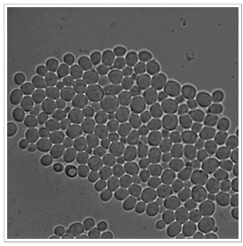
Currently ten test sets (TS) have been extracted and they cover the basic situations such as:
- single cells and small colonies (TS1, TS2, TS6, TS9 and TS10)
- colony translations and merging (TS3)
- big colonies with heavily clustered cells (TS4, TS5, TS7, TS8)
Ground truth
In order to perform automatic evaluation of the algorithm, the ground truth is required. For each TS it was prepared in a manual manner by one of the authors and then verified and corrected by the rest of the team. The resulting ground truth includes cell center locations, unique cell number throughout the TS and "facultative tag". Facultative tag is used to mark the cells on the edge of images (some algorithms discard them by design) and objects which we find questionable. The algorithm is not penalized for discovering / ommiting the cells marked as facultative.
Overview
The following table summarises the test sets:
| Test set | Start time | Frame count | Cell number span | Animation |
|---|---|---|---|---|
| TS1 | 1 | 60 | 14 - 26 |  |
| TS2 | 1 | 30 | 4 - 6 |  |
| TS3 | 191 | 20 | 101 - 128 |  |
| TS4 | 225 | 20 | 171 - 237 |  |
| TS5 | 180 | 20 | 140 - 173 |  |
| TS6 | 65 | 10 | 36 - 49 |  |
| TS7 | 150 | 10 | 129 - 184 |  |
| TS8 | 1 | 30 | 60 - 88 |  |
| TS9 | 1 | 30 | 41 - 68 |  |
| TS10 | 1 | 30 | 16 - 16 |  |
Principles of the state of the art algorithms
Cell segmentation and tracking are widely studied problems and have been approached in many different ways. Shen et. in 2006 presented Active Contours segmentation approach applied to fluorescence images combined with particle filter tracking (Shen2006). Kvarnstroem et al. in 2008 approached yeast cells segmentation in bright field images using a combination of circular Hough transform and dynamic programming performed on polar plots (Kvarnstroem2008). Zhou et al. in 2009 proposed markov models for segmentation and cell phase identification in fluorescence microscopy (Zhou2009). Delgado-Gonzalo et al. in 2010 introduced probabilistic formulation of tracking on bipartite graphs and cell motion model dependent on neighbour cells moves (Delgado2010). Sansone et al. in 2012 combined circular hough transform with machine-learning based false positives detection for segmentation in phase-contrast microscopy and presented evaluation of the algorithm using precision and recall measurements (Sansone2012).
In 2019 we added the novel algorithm by Wood et. al (Wood2019). We would like to thank authors for providing both the description and partial results. It jointly segment and track each invidual cell from last frame to the first using multiple watershed thresholds.
Here we present in details, seven chosen as best fitting our needs, algorithms for segmentation and tracking of yeast cells in bright field microscopy: CellID (Gordon2007), Intensity Based Segmentation - Overlap Based Tracking via CellProfiler (IBSOBT) (Carpenter2006), CellTracer (Wang2009), Tracker (Uhlendorf2012), CellSerpent (Bredies2011), Wood (Wood2019).
| Program | Webpage | Publication |
|---|---|---|
| Cell Tracer | http://www.stat.duke.edu/research/software/west/celltracer/ | (Wang2009) |
| CellID | http://lbms.df.uba.ar/ | (Gordon2007) |
| CellProfiler | http://cellprofiler.org/ | (Carpenter2006) |
| Tracker | upon req. | (Uhlendorf2012) |
| Cell Serpent | http://microscopy.uni-graz.at/index.php?item=new2 | (Bredies2011) |
| Cell Star | http://cellstar-algorithm.org/ | (Versari2017) |
| Wood | https://journals.plos.org/plosone/article?id=10.1371/journal.pone.0206395 | (Wood2019), (Doncic2013) |
Cell Tracer
Automated image analysis presented in CellTracer uses an iterative approach for combining a set of morphological operations to perform segmentation on Bright-field (as well as fluorescent) images. Segmentation process consists of two main steps: pre-processing and cell identification itself. For purposes of this approach there was invented concept of black-white/gray-scale hybrid images - that means reserving extreme values (0 and 255) for special purposes eg. marking background or borders
Preprocessing
Preprocessing performs three-class partitioning of the images into: background regions, border regions and yet to be decided.
Background identification
Background identification is made using a modified non-linear range filter with a disk-shaped structure element. With an assumption that cells are rather smooth-shaped the radius of this element is determined as value in between r and 2r where r is estimated as maximum cell half-width among all processed images. After application of this filter image is thresholded with fixed value (user input), so pixels with values below certain level are marked as background. The filter application is then followed by morphological dilation.
Border identification
Borders are identified using high-pass range filter. It also has disk-shaped structure element. The second significant change to default filter is that background pixels from previous step are not considered as minimum values within the neighborhood of processing pixel. For this step there is also a threshold value assuring that only obvious borders are marked - as maximum values (255) - on the hybrid image.
Cell identification
The second and main step is identification of cells in preprocessed hybrid image. It is achieved in following steps:
- Labelling disconnected blobs (disconnected segmented regions)
- Filtering each labelled blob using hybrid filters or a combination of filters, to erode the undecided regions, followed by hybrid dilation and smoothing to restore most of the pixel values changed by the filter- it leads usually to breaking down blobs into smaller ones.
- Scoring blobs based on cell model assumptions – score in two criterions:
- Cell shape - cell shapes are assumed to be convex or almost convex. Score is computed as difference between blob area and blob convex area divided by blob perimeter
- Cell intensity value distribution - interior cell regions are assumed to be relatively darker than border regions.
- Dividing blobs into two subsets - these with higher score and these with lower score
- Repeating steps 1-4 for cells with higher scores
CellID
This program was developed around the observation that images of yeast cells that are taken slightly out of focus have a very distictive dark rim around them. It makes it fairly simple to find these edges using adaptive thresholding. However in this work that specific type of imagery is not available but we will try to compensate for it with the proper preprocessing.
Cell segmentation:
Dark boundary pixels are found using thresholding with cutoff value calculated as the mean of the distibution minus a number of standard deviation. Then cells are defined as the contiguous regions separated by these boundary pixels. The next step is filtering out the regions which sizes are outside a specified range. These preliminary results of the segmentation are then processed using simple heuristics that can split up two joined cells.
Tracking:
The newly found cells are compared with cells from previous frame based on their geometrical overlap defined as intersection over union of the cells regions. The new cell is matched with the one with the highest value only if it is above the user-defined cut off.
Intensity Based Segmentation Overlap Based Tracking (IBSOBT) via CellProfiler
Processing image sequence in CellProfiler proceeds as follows:
Pre-processing:
The first step is preprocessing image. It uses three types of images: smoothed input image, thresholded and smoothed edges image, and image with convex hull-smoothed illumination correction. Cell interiors intensities are increased by combining illumination correction image with original image, then border intensities are decreased by subtracting smoothed and thresholded edges.
Cell segmentation:
CellProfiler contains a modular three-step strategy to identify objects even if they touch each other.
- CellProfiler determines whether an object is an individual nucleus or two or more clumped nuclei.
- The edges of nuclei are identified, using thresholding if the object is a single, isolated nucleus, and using more advanced options if the object is actually two or more nuclei that touch each other (Wahlby, 2004).
- Some identified objects are discarded or merged together if they fail to meet certain your specified criteria. For example, partial objects at the border of the image can be discarded, and small objects can be discarded or merged with nearby larger ones.
Tracking:
When trying to track an object in an image, CellProfiler will search within a maximum specified distance of the object's location in the previous image, looking for a "match". Objects that match are assigned the same number, or label, throughout the entire image sequence. Here we use overlap approach that compares the amount of spatial overlap between identified objects in the previous frame with those in the current frame. The object with the greatest amount of spatial overlap will be assigned the same number (label).
'Tracker'
This is an algorithm used by Uhlendorf et al. 2012 which represents model-based approach. It assumes that yeast cells are circluar in shape and therefore looks for potential circles in the image.
Preprocesing:
First the gradient field of the input image is calculated which is then thresholded to leave only pixels that are supposed to belong to the borders of the cells.
Cell segmentation:
The circular Hough Transform is used to determine the positions and radiuses of the circles representing cells. Every pixel 'votes' for all the circles it can belong to and after accumulation of all the votes the circles with locally highest vote count are chosen.
Tracking:
The cells recognized in the current image are compared with the ones from the last (or last but one if the gap is detected) image. Linear optimization is used to match the cells using a defined cell-to-cell distance matrix.
CellSerpent
Implementation of an algorithm described by K. Bredies and H. Wolinski in (Bredies2011). The main idea behind this approach is to adapt Active Contours algorithm for cell segmentation purpose.
Preprocessing
Preprocessing contains three steps:
- Background normalization
- Background detection
- Computing non-linear elliptic degenerate denoising
Segmentation
Seeding
This part of algorithm finds start points for Active Contours algorithm - "seeds" from which cells are grown up. This is done by finding the local maxima for a smoothed edge-penalization image. Local maximum usually corresponds to point in the center of a cell. Points obtained by this procedure are clustered to ensure that a minimum distance is preserved and returned after checking that none of the points lies in the previously determined cell-free-region mask.
Cell detection
This step requires its own computation of edge-penalization images for both original image and smoothed image. Additional penalization is added for the cell-free regions in order to avoid the active contour entering there. For each seed from previous step an active contour is initiated around it and evolved according to the optimization problem with edge-penalization image obtained from smoothed image. After meeting the stopping criterion, the procedure is repeated with the edge-penalization image obtained from original image and returns the contour of the cell.
Postprocessing
After the contour tracing is finished, the method creates a label image which assigns each pixel a positive natural number unique to each cell and 0 to the background. Starting with the contour associated with the lowest functional value for optimization problem, the region occupied by the contour is determined and checked against the label image for intersection. If the area of intersection is too large, the current region is rejected, otherwise, it is incorporated into the label image with a new number. In the resulting label image, each cell can be identified through the corresponding pixels.
CellSerpent*
We use this designation for our modification of CellSerpent algorithm. This modification includes slightly changes that improved results we obtained compared to original version. The changes include following:
- Enchanced background detection
- Edge continuity enchancement preventing seeds falling directly between two cells
CellStar
Preprocessing
In this step a background image is prepared - either predefined or manually chosen and adjusted to remove areas occupied by cells. Processed image is divided according to background image into two parts:
- pixels darker than background and its median filtered version
- pixels brighter than background and its median filtered version
Foreground content-border segmentation
Foreground regions are determined for processing image as areas where difference of values between image and background is relatively big. Then foreground is enchanced with two-step hole filling and splited into two parts - content and border
- darker part is cell content
- brighter part is cell border
Seed and grow snakes
In few steps - first find big cells then try to find smaller.
Find new seeds (depends on parameters)
Based on cell content or border pixels (potentially excluding already segmented regions) and previous computations
- find local minimas
- cluster minimas (from CellSerpent?)
- centroids of previous snakes
Grow new seeds into snakes
Prepare uniformly distributed rays from seed position
- for different length of rays calculate its properties
- choose best length for every arc
- starting from the best arc drop the consecutive ones if the distance too big
- unstick edge points?
- an additional smoothing?
- calculate best snake properties
Filter snakes list
- sort snakes by rank
- remove snakes with too high rank
- trim snake to regions free from better snakes
- recalculate properties and remove snake if not good enough
Tracking
Find cell detection data
Collect all the centroid and size data from segmentation
Find initial cell tracks
Uses min-cost assignment (Hungarian) based on distance and size
Improve results in a few iteration
- ComputeDetailedMotion
- ComputeMotionByFrames
- GetLocalizedPrimitiveTracks
Wood
Ezgi Wood provided us with the description of the solution. The algorithm’s implementation in MATLAB is available as a supplementary material at the journal website.
The algorithm starts with segmenting the last image of a time series and segments images backwards in time by using the segmentation of the previous time point as a seed for segmenting the next time point.
Seeding last time point
The image of the last time point is automatically segmented by a two-step automated seeding algorithm: First, the image is pre-processed and watershed algorithm is applied to the processed image to generate coarse seeds. Next, the algorithm automatically fine-tunes these coarse seeds and automatically detects and corrects segmentation mistakes (Wood2019).
Stable cell contour
Next, given a seed for the cell, the algorithm focuses on a subimage containing the seed. First, the algorithm creates a series of binary images by applying every possible threshold for an 8-bit image. The watershed algorithm is applied to all these binary images and regions that significantly overlap with the seed are combined in a composite image that allows for more accurate segmentation than one optimized threshold (Doncic2013).
Tracking
The cells are tracked based on their overlap with their seed.
Input data assumptions
Every algorithm has to make some assumptions about the input data and what cells generally look like so it can utilize this in cell segmentation. We sum up these basic assumptions in the following table:
| IBSOBT via CellProfiler | CellTracer | CellID | Tracker | CellSerpent | CellStar | ! Wood |
|---|---|---|---|---|---|---|
| Bright and thick borders | Brighter borders, darker content / background * | Dark borders | High gradient borders | High gradient borders | Brighter borders, darker content compared to background | Brighter borders, darker content ** / background |
*There is a possibility to invert input values in CellTracer's GUI. **If the content is not dark, a composite image of phase and fluorescent image can be used for segmentation.
Specification of dataset adjustments and tool configurations
The comparison of the existing tools poses a couple of challenges. In the case of image processing, the results of the algorithms are highly dependent on the data used. It is even possible that simpler and theoretically worse one can perform better than the complex ones in case of very noisy input images.
Another problem is that the tools that we compare are configurable so the question arises: is the chosen configuration optimal? Furthermore algorithms may require suitable preprocessing to enhance the features that they use. It means that there is not only a need to test different configurations but also different preprocessing. That's why it is not obvious how to provide fair comparison of such algorithms.
Our solution is to start the search for the best preprocessing-configuration pair using the remarks in the corresponding papers. Then for every test set we try to adjust the parameters to produce better results.
The following sections describe both the preprocessing used and how the 'optimal' configurations were determined.
Cell Tracer
Image preprocessing:
Contrast enhancement.
Configuration determination:
Optimal configuration was obtained by choosing right combination of small predefined set of methods grouped by purpose (background detecition, border detection, cell identification, tracking) and first of all adjusting their parameters. Configuration combined methods in this group order. For each method there were adjusted specific parameters until the output result was satisfying. Methods in groups was tested in different orders to find the best solution. Tests were performed on 2-3 images per data set and results was visually tested to meet requirements. We used the possibility to save 'snapshots' after obtaining good results for one method to avoid repeating the whole sequence of previously adjusted methods before each parameter change in currently tested method.
CellID
Image preprocessing:
Smooting, invertion, contrast enchancement, unsharp filter, (opt minimum morphology).
Configuration determination:
This tool is designed for out-of-focus images which is not the case here so we need to mimic its characteristics with proper preprocessing. In order to create dark rims we invert the image and to enchance their size we use the combination of constrast enchancement and unsharp filter. In case of the test sets with highly clustered cells we additionally apply minimal morphology for better separation.
The optimal parameters were chosen per data set using one of its images. First the acceptable cell size was selected so that every possible cell is valid and the small incorrect ones are filtered out. Then the background reject factor and the rest of the parameters were trimmed to find the balance between separation of clustered cells and oversegmentation of the existing ones.
IBSOBT via CellProfiler
Image preprocessing:
Smoothing, contrast enchancement, edge enchancement.
Configuration determination:
Optimal configuration was obtained during two stages - local and global. Both stages were performed on 2-3 images. In first stage, for each module in pipeline, resulting output was visually compared to expecting output, and parameters were corrected until satisfying output was obtained. In second parameters were adjusted for better results in other modules, especially the final ones - segmentation and tracking.
'Tracker'
Image preprocessing:
Contrast streach
Configuration determination:
Optimal configuration was obtained by choosing the right parameters - preprocessing combination. In order to do so the tested image had been variously preprocessed (median filter, contrast streach, equalization). For every data set the image that was the most challenging for the default parameters was used to trim the parameters. First the sensible cell size range was set. Then the threshold and filter radius parameters were trimmed until the best results were obtained.
CellSerpent
Image preprocessing:
Edge enchancement
Configuration determination:
Optimal parameters were determined for each stage separately and then confirmed to work good combined together. This was done by visual rating results of image smoothing, background determination and seeding followed by both visual and automatic evaluation of Active Contour algorithm.
CellStar
Image preprocessing:
None (for our test sets).
Configuration determination:
Default configuration
Wood
Algorithm was applied to test sets TS1-2, TS6, TS8-10.
Image preprocessing:
Bright field images were first corrected for uneven background by subtracting a gaussian filtered image from the image. Next, tophat transformation was applied. For TS8, the complements of the bright field images were used. Phase images were not processed.
Configuration determination:
Optimal configuration was obtained by choosing the right processing for bright field images and by optimizing the parameters for the objective magnification and imaging conditions. Bright field images were processed to make the borders brighter than cell centers and background. To optimize the parameters the last image of the time series was used. It was first segmented with the default parameters and then parameters were adjusted until getting a satisfying output. For the implementation of processing and the values of the parameters used see (Wood2019).
Result of the comparison
Visual inspection:
The first method of comparison is visual inspection. In order to make more accurate and convenient we put all the results in the 3 by 2 grid.
Undersegmentation
Undersegmetation appears in almost every tested program (only one exception - 'Tracker'). It is a state when region detected as one cell contains areas belonging to few cells. It is very rare for every program it appeared in.

Examples of undersegmentation
Oversegmentation
Oversegmentation similiary appears in every program except 'Tracker'. In contrary to undersegmentation it is a state when a cell is detected as few cells. It is rare for CellStar and CellSerpent. More often it appears in IBSOBT then CellTracer. The most susceptible to oversegmentation is CellID.

Examples of oversegmentation
False positives
There is no false-positive-free program. However 'Tracker' and CellStar have very little number of false positives - accidentally found in the noisy background. CellTracer and IBSOBT detect false positives in areas between groups of cells, CellID find lots of cells in noisy background and CellSerpent suffers from inexact background detection causing seeds to fall out of area covered by cells.

Examples of false positives
False negatives
False negatives are one of most crucial obstacles in further cell processing. There is one definite leader in low number of false negatives - CellStar. It omits cells most rarely, CellTracer however is also doing well. Other programs occur to produce more false negatives (especially IBSOBT) whatt is most probably caused by inconsistent cell interiors.

Examples of false negatives
Cell contour extraction accuracy
Cell contour extraction techniques used in tested programs are different, however in most cases they are extracted quite accurately. Only one exception is Tracker which uses Circular Hough Transform and therefore extract cell contours as circles.

Examples of cell contours extraction
Detection of cells near image boundaries
Due to specific image processing techniques some programs are suffering from missing cells near image boundaries. CellTracer has least problems with this issue. Tracker and CellSerpent are also coping with it quite well.

Detection of cells near image boundaries
Detection rate for new cells
Detection of new cells is probably the most important issue from lineage analysis' point of view. CellStar has the best results among all tested programs. The only one problem can be that technique ensuring early detection of new cells probably causes over segmentation in some cases. CellTracer is almost as good, however the side effect in this case is false positive detection. CellID and CellSerpent detect new cells in reasonable time, but no as fast as programs mentioned above. Tracker and IBSOBT perform very poor - Tracker has 5 frames latency compared to CellStar, and IBSOBT has even more as shown below.

Detection of new cells
Tracking errors
There is no program that tracks cells perfectly - example below shows very challenging situation in which none of tested programs track cells without errors. CellSerpent does not provide cell tracking, thus there is no visual result for it.

A problematic situation for tracking
Summary
It is apparent that none of the algorithms is perfect all of them misses some parts of cells. The most successful is CellStar because it marks almost every cell and almost never finds cell where there isn't one, when the rest can't deal with the clustered cells and spaces between cell groups. It has also the best budding cells detection rate together with CellTracer. On the other hand CellTracer is just only algorihm that has no problems with detecting cells near image boundaries.
Automatic evaluation:
However manual evaluation should always be supplemented by automatic evaluation. In this case both the results of segmentation and tracking can be tested against the manually created ground truth. First thing to do is to find the correspondence between the ground truth cells and the cells in the output of the algorithm. This can be achieved using simple nearest neighbour method or more sophisticated LP (Sansone, 2011).
Quality measures:
There is a number of principally similar segmentation quality measures:
- False positive/negative (Bao, 2007)
- Oversegmentation/undersegmentation (Waleby, 2004 and Zhoul, 2006/9)
- Precision/recall (Sansone, 2011)
A false-positive is a cell that is recognized by the algorithm but does not exist in the ground truth. A false-negative is a cell that the algorithm missed. All the rest is simply a variation of that. Precision and recall measures are used in this work as they are normalized by the total cell number. It is important to always consider both measures because the algorithm can always be trimmed to increase one of them in cost of the other.
Precision and recall calculation method:
Let R be the set of cells in the results, G be the set of cells in the ground truth and C be the set of correspondence pairs between R and G. Then:

F is an additional quality measure (combining precision and recall).
The above measures test only the ability of the algorithm to find the centers of cells so to evaluate the accuracy we can calculate the overlap of the corresponding contours (Sansone, 2011). However in this paper it is done by visual inspection.
Facultative ground truth:
There are some inconclusive objects in the images and the algorithms should not be penalised nor rewarded for finding them, otherwise it would clutter the results.
Let  be the set of cells in the ground truth marked as facultative.
Then:
be the set of cells in the ground truth marked as facultative.
Then:

Precision and recall can then be properly adjusted:
Tracking evaluation
Performance of the tracking algorithm in each image can be evaluated using similar precision and recall measures based on the number of correct links (Primet, 2011). A link is two consecutive points in a cell trajectory. Thus a correct link is the case when algorithm finds both points of the link in the ground truth and recognize that they belong to the same cell..
Precision, recall and F is calculated analogous to the segmentation but with:
= the subset of C where at least one end is marked as facultative
Another measure for tracking performance is long-term tracking which evaluates the ability of the algorithm to correctly track cells throughout the whole image series. For this purpose we adapt the tracking measure defined above. It is calculated for the set of only two images (first and last).
Evaluation platform:
The previous section presented measures viable for evaluation of image segmentation and tracking. In order to apply the above measures to test sets we created evaluation and comparison software called Evaluation platform (available to download). The platform is written in Python which makes it easily portable (tested on Windows and Mac OX) and has simple API so it is easy to configure and use. The details of API and examples of usage are provided in the documentation included with the software.
The evaluation is presented with precison-recall-F plots for both segmentation and tracking. Additionally, it can plot the details of the evaluation such as the correct/incorrect cells on the input images. Evaluation platform is independent from yeast problem and can be used to analyze any tracking algorithm.
Results:
Test set 3 is very challenging for tracking algorithm due to sudden merge of three different colonies of yeast cells so we start with this one. First, lets examine the segmentation performance. All the algorithms performed well with more than 85% of the cells found and precision factor over 90%. The best results were achieved by CellStar with over 95% of cells detected and almost all of the returned cells were correct.

Segmentation evaluation in TestSet3.
In the case of this test set tracking evaluation is much more interesting. It is clear from the plots when movement occurs. Only CellStar is able (partially) to cope with this situation because all of the other algorithms use overlap or distance between cells to track them which in this case is meaningless. Better solution would use cell based characteristics such as size, shape (Zhou, 2006, 2011) or even intensity histogram. Another improvement would be taking into account the relative position between cell and its neighbours because it usually does not change dramatically which is something that CellStar uses.

Tracking evaluation in TestSet3.
Table summarising segmentation quality (F measure) in all TestSets (green - best; blue - second best, NE - not evaluated):
| Test set | IBSOBT | CellTracer | CellID | Tracker | CellSerpent* | CellStar | Wood |
|---|---|---|---|---|---|---|---|
| TS1 | 0.8847 | 0.9239 | 0.6302 | 0.9351 | 0.9712 | 0.9921 | 0.9894 |
| TS2 | 0.8923 | 0.9071 | 0.3073 | 0.9531 | 0.9677 | 0.9895 | 1.0000 |
| TS3 | 0.9094 | 0.9331 | 0.9356 | 0.9176 | 0.9349 | 0.9852 | NE |
| TS4 | 0.8238 | 0.9362 | 0.9297 | 0.8960 | 0.9065 | 0.9797 | NE |
| TS5 | 0.9023 | 0.9452 | 0.9209 | 0.9036 | 0.9045 | 0.9728 | NE |
| TS6 | 0.7835 | 0.7374 | 0.7774 | 0.8671 | 0.8704 | 0.9618 | 0.9698 |
| TS7 | 0.8837 | 0.8740 | 0.7805 | 0.8861 | 0.9008 | 0.9610 | NE |
| TS8 | NE | NE | NE | NE | NE | NE | 0.9862 |
| TS9 | NE | NE | NE | NE | NE | NE | 1.0000 |
| TS10 | NE | NE | NE | NE | NE | NE | 1.0000 |
Table summarizing tracking quality (F measure) in all TestSets (green - best; blue - second best, NE - not evaluated):
| Test set | IBSOBT | CellTracer | CellID | Tracker | CellSerpent* | CellStar | Wood |
|---|---|---|---|---|---|---|---|
| TS1 | 0.8393 | 0.9109 | 0.6164 | 0.9339 | NA | 0.9928 | 0.9901 |
| TS2 | 0.7184 | 0.9020 | 0.3361 | 0.9545 | NA | 0.9853 | 1.0000 |
| TS3 | 0.8709 | 0.8750 | 0.9100 | 0.8953 | NA | 0.9802 | NE |
| TS4 | 0.7839 | 0.8713 | 0.8964 | 0.8589 | NA | 0.9715 | NE |
| TS5 | 0.8940 | 0.9015 | 0.9015 | 0.8888 | NA | 0.9771 | NE |
| TS6 | 0.7196 | 0.5413 | 0.7516 | 0.8619 | NA | 0.9608 | 0.9783 |
| TS7 | 0.8363 | 0.7939 | 0.6512 | 0.8716 | NA | 0.9549 | NE |
| TS8 | NE | NE | NE | NE | NE | NE | 0.9899 |
| TS9 | NE | NE | NE | NE | NE | NE | 1.0000 |
| TS10 | NE | NE | NE | NE | NE | NE | 1.0000 |
Table summarising long-time tracking quality (F measure) in all TestSets (green - best; blue - second best, NE - not evaluated):
| Test set | IBSOBT | CellTracer | CellID | Tracker | CellSerpent* | CellStar | Wood |
|---|---|---|---|---|---|---|---|
| TS1 | 0.0000 | 0.4211 | 0.2857 | 0.9167 | NA | 1.0000 | 1.0000 |
| TS2 | 0.5000 | 0.3333 | 0.4444 | 1.0000 | NA | 1.0000 | 1.0000 |
| TS3 | 0.4460 | 0.3649 | 0.6587 | 0.6905 | NA | 0.8776 | NE |
| TS4 | 0.5076 | 0.3981 | 0.5517 | 0.5767 | NA | 0.8922 | NE |
| TS5 | 0.7821 | 0.4526 | 0.8000 | 0.8176 | NA | 0.9670 | NE |
| TS6 | 0.4091 | 0.2439 | 0.6415 | 0.9180 | NA | 1.0000 | 0.9873 |
| TS7 | 0.5399 | 0.4471 | 0.5590 | 0.8800 | NA | 0.9167 | NE |
| TS8 | NE | NE | NE | NE | NE | NE | 1.0000 |
| TS9 | NE | NE | NE | NE | NE | NE | 1.0000 |
| TS10 | NE | NE | NE | NE | NE | NE | 1.0000 |
Downloads
References
- (Ambuehl2011): High-resolution cell outline segmentation and tracking from phase-contrast microscopy images, Ambuehl et al., Journal of Microscopy 2011.
- (Bredies2011): An active-contour based algorithm for the automated segmentation of dense yeast populations on transmission microscopy images, Bredies et al., 2011.
- (CellProfilerManual): CellProfiler online manual: http://www.cellprofiler.org/CPmanual/
- (Carpenter2006): CellProfiler: image analysis software for identifying and quantifying cell phenotypes, Carpenter et al., 2006.
- (Delgado2010): Multi-target tracking of packed yeast cells. G. R. Delgado et al. Biomedical Imaging: From Nano to Macro
- (Gordon2007): Single-cell quantification of molecules and rates using open-source microscope-based cytometry, Gordon et al., Nature Methods, 2007.
- (Held2010): Cellcognition: time-resolved phenotype annotation in high-throughput live cell imaging, Held et al., Nature Methods, 2010.
- (Kvarnstroem2008):Image analysis algorithms for cell contour recognition in budding yeast, Kvarnström et al, Opt. Express 16, 2008
- (Primet2011): Probabilistic methods for point tracking and biological image analysis, Mael Primet, 2011.
- (Sansone2011): Segmentation, tracking and lineage analysis of yeast cells in bright field microscopy images, Sansone et al., 2011.
- (Shen2006): Automatic tracking of biological cells and compartments using particle filters and active contours, Shen et al. 2006, Chemometrics and Intelligent Laboratory Systems.
- (Uhlendorf2012): Long-term model predictive control of gene expression at the population and single-cell levels, Uhlendorf et al., PNAS, 2012.
- (Versari2017): Long-term tracking of budding yeast cells in brightfield microscopy: CellStar and the Evaluation Platform Versari et al., Journal of the Royal Society Interface, 2017.
- (Wang2008): CellTracer: Software for automated image segmentation and lineage mapping for single-cell studies, Wang et al., 2008.
- (Wang2009): Image segmentation and Dynamic Lineage Analysis in Single-Cell Fluorescence Microscopy, Wang et al., 2009.
- (Wahlby2004): Combining intensity, edge and shape information for 2D and 3D segmentation of cell nuclei in tissue sections, Wahlby et al., J Microsc, 2004.
- (Yao2004): A Multi-Population Genetic Algorithm for Robust and Fast Ellipse Detection, Yao et al., 2004.
- (Zhou2006): Automated segmentation, classification, and tracking of cancer cell nuclei in time-lapse microscopy, Zhou et al., TBE, 2006.
- (Zhou2009): A Novel Cell Segmentation Method and Cell Phase Identification Using Markov Model, Zhou et al., TITB, 2009.
- (Wood2019) Wood, N. E., & Doncic, A. (2019). A fully-automated, robust, and versatile algorithm for long-term budding yeast segmentation and tracking. PloS one, 14(3), e0206395.
- (Doncic2013) Doncic, A., Eser, U., Atay, O., & Skotheim, J. M. (2013). An algorithm to automate yeast segmentation and tracking. PLoS one, 8(3), e57970.
Additional related papers can be found here.